---
title: "Pivekimab Sunirine in Blastic Plasmacytoid Dendritic Cell Neoplasm"
subtitle: "A Visual Summary of the CADENZA Phase I/II Trial"
author:
- name: "Based on Pemmaraju N, Marconi G, Montesinos P, et al."
affiliation: "*J Clin Oncol* 2026; DOI: 10.1200/JCO-25-02083"
date: today
format:
html:
theme: journal
toc: true
toc-depth: 3
toc-location: right
number-sections: true
code-fold: true
code-tools: true
code-summary: "Show code"
fig-align: center
fig-width: 10
fig-height: 7
fig-dpi: 300
smooth-scroll: true
mainfont: "Helvetica Neue"
fontsize: "1.05em"
title-block-banner: "#1a5276"
title-block-banner-color: white
execute:
warning: false
message: false
echo: true
bibliography: references.bib
---
::: {.callout-note appearance="minimal"}
## Key Findings at a Glance
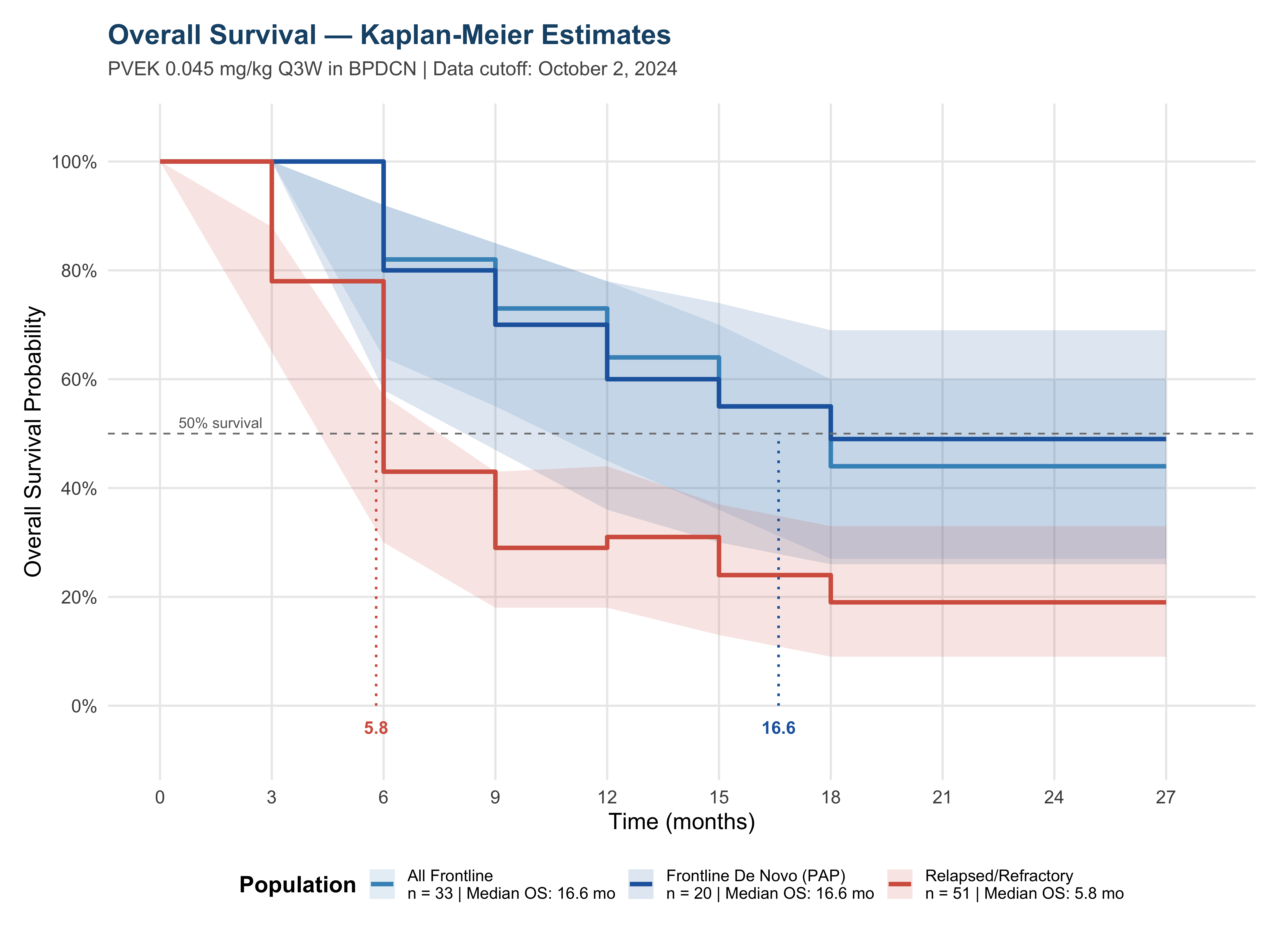
**Pivekimab sunirine (PVEK)** — a first-in-class CD123-targeted antibody–drug conjugate — achieved a **75% composite complete response (CCR)** rate in frontline de novo BPDCN, with median overall survival of **16.6 months**, and a manageable safety profile.
:::
# Background {#sec-background}
* Blastic plasmacytoid dendritic cell neoplasm (BPDCN) is an ultra-rare (≈0.05 per 100,000), aggressive hematologic malignancy involving skin, bone marrow, blood, lymph nodes, and CNS.
* It is characterized by universal overexpression of CD123 (interleukin-3 receptor-α) on neoplastic blasts, making CD123 an attractive therapeutic target.
* The median age at diagnosis is approximately 65 years, with a 3:1 male predominance.
* Until recently, treatment options were largely limited to chemotherapy regimens adapted from acute leukemias, with historically poor outcomes.
* **Tagraxofusp**, a CD123-directed cytotoxin, became the first and only approved targeted therapy for BPDCN.
* The CADENZA trial (NCT03386513) evaluated a novel approach: **pivekimab sunirine (PVEK)**, a CD123-targeted antibody–drug conjugate.
## Mechanism of Action
```{r}
#| label: fig-mechanism
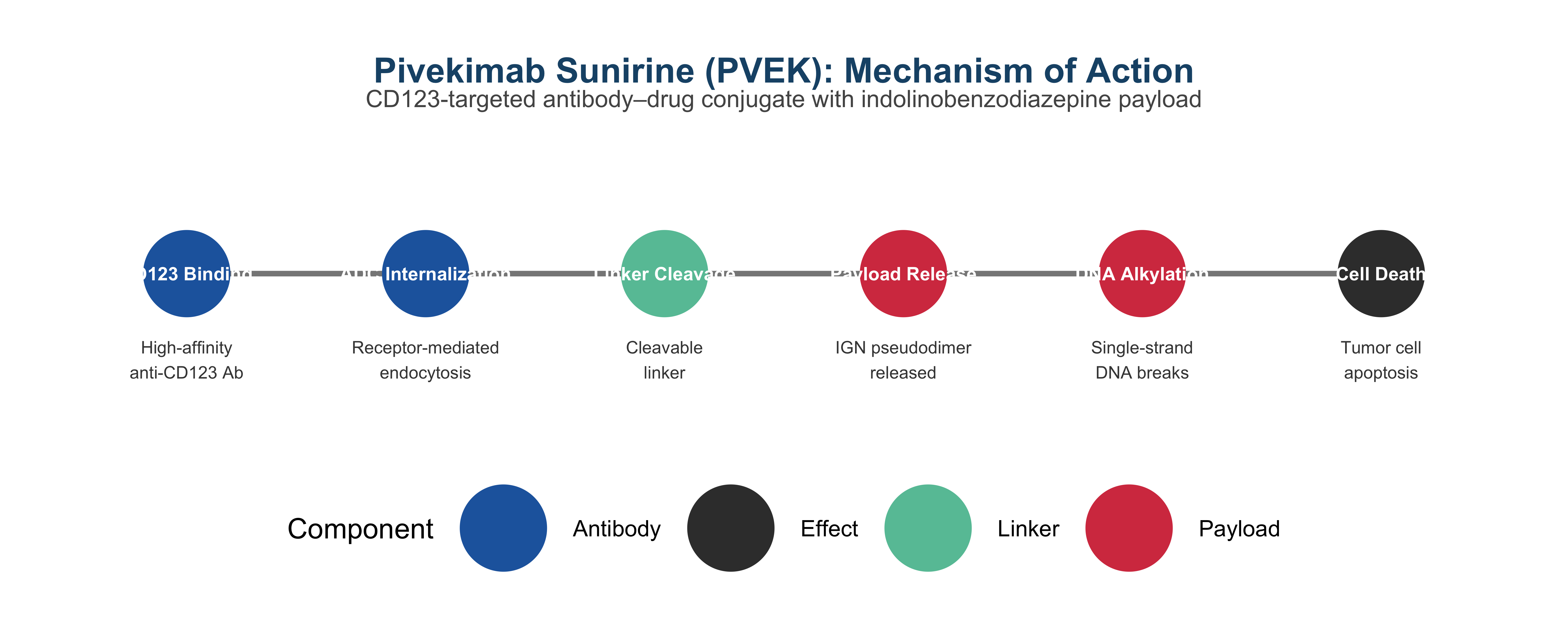
#| fig-cap: "Schematic overview of PVEK mechanism: anti-CD123 antibody binds to CD123 on BPDCN blasts, delivering an indolinobenzodiazepine pseudodimer payload that alkylates DNA and causes single-strand breaks."
#| fig-height: 4
#| code-fold: true
library(ggplot2)

# Create a conceptual diagram of the ADC mechanism
mechanism_data <- data.frame(
  step = factor(c(
    "1. CD123\nBinding",
    "2. ADC\nInternalization",
    "3. Linker\nCleavage",
    "4. Payload\nRelease",
    "5. DNA\nAlkylation",
    "6. Cell\nDeath"
  ), levels = c(
    "1. CD123\nBinding",
    "2. ADC\nInternalization",
    "3. Linker\nCleavage",
    "4. Payload\nRelease",
    "5. DNA\nAlkylation",
    "6. Cell\nDeath"
  )),
  component = c("Antibody", "Antibody", "Linker", "Payload", "Payload", "Effect"),
  y = c(1, 1, 1, 1, 1, 1),
  description = c(
    "High-affinity\nanti-CD123 Ab",
    "Receptor-mediated\nendocytosis",
    "Cleavable\nlinker",
    "IGN pseudodimer\nreleased",
    "Single-strand\nDNA breaks",
    "Tumor cell\napoptosis"
  )
)

color_palette <- c(
  "Antibody" = "#2166ac",
  "Linker"   = "#66c2a5",
  "Payload"  = "#d53e4f",
  "Effect"   = "#3a3a3a"
)

ggplot(mechanism_data, aes(x = step, y = y)) +
  geom_segment(
    data = data.frame(x = 1:5, xend = 2:6, y = 1, yend = 1),
    aes(x = x, xend = xend, y = y, yend = yend),
    inherit.aes = FALSE,
    arrow = arrow(length = unit(0.25, "cm"), type = "closed"),
    color = "#888888", linewidth = 1.2
  ) +
  geom_point(aes(color = component), size = 18) +
  geom_text(aes(label = gsub("\\d+\\. ", "", gsub("\n", " ", as.character(step)))),
            size = 3, fontface = "bold", color = "white") +
  geom_text(aes(label = description, y = y - 0.15),
            size = 2.8, color = "#444444") +
 scale_color_manual(values = color_palette, name = "Component") +
  scale_x_discrete() +
  scale_y_continuous(limits = c(0.7, 1.2)) +
  labs(
    title = "Pivekimab Sunirine (PVEK): Mechanism of Action",
    subtitle = "CD123-targeted antibody–drug conjugate with indolinobenzodiazepine payload"
  ) +
  theme_void(base_size = 13) +
  theme(
    plot.title = element_text(hjust = 0.5, face = "bold", size = 16, color = "#1a5276"),
    plot.subtitle = element_text(hjust = 0.5, size = 11, color = "#555555",
                                 margin = margin(b = 15)),
    legend.position = "bottom",
    plot.margin = margin(20, 20, 20, 20)
  )
```
# Study Design {#sec-design}
The CADENZA trial was an international, phase I/II, open-label, multicenter study. Patients received PVEK **0.045 mg/kg once every 3 weeks** (day 1 of a 21-day cycle) as a ≤30-minute infusion.
::: {.panel-tabset}
## Populations
| Population | Description | N |
|:-----------|:------------|--:|
| **PAP** (Primary Analysis) | Frontline de novo BPDCN | 20 |
| **All Frontline** | De novo + PCHM | 33 |
| **Relapsed/Refractory** | 1–3 prior systemic therapies | 51 |
| **Total** | All BPDCN patients | 84 |
## Key Endpoints
| Endpoint | Type | Definition |
|:---------|:-----|:-----------|
| **CCR rate** | Primary | CR + CRc per investigator assessment (PAP) |
| **Duration of CCR** | Key Secondary | Time from first CCR to relapse/death |
| **OS** | Secondary | Time from first dose to death |
| **ORR** | Secondary | CR + CRc + CRh + CRi + PR |
| **Bridge to SCT** | Exploratory | Patients proceeding to stem-cell transplant |
:::
# Patient Demographics {#sec-demographics}
```{r}
#| label: fig-demographics
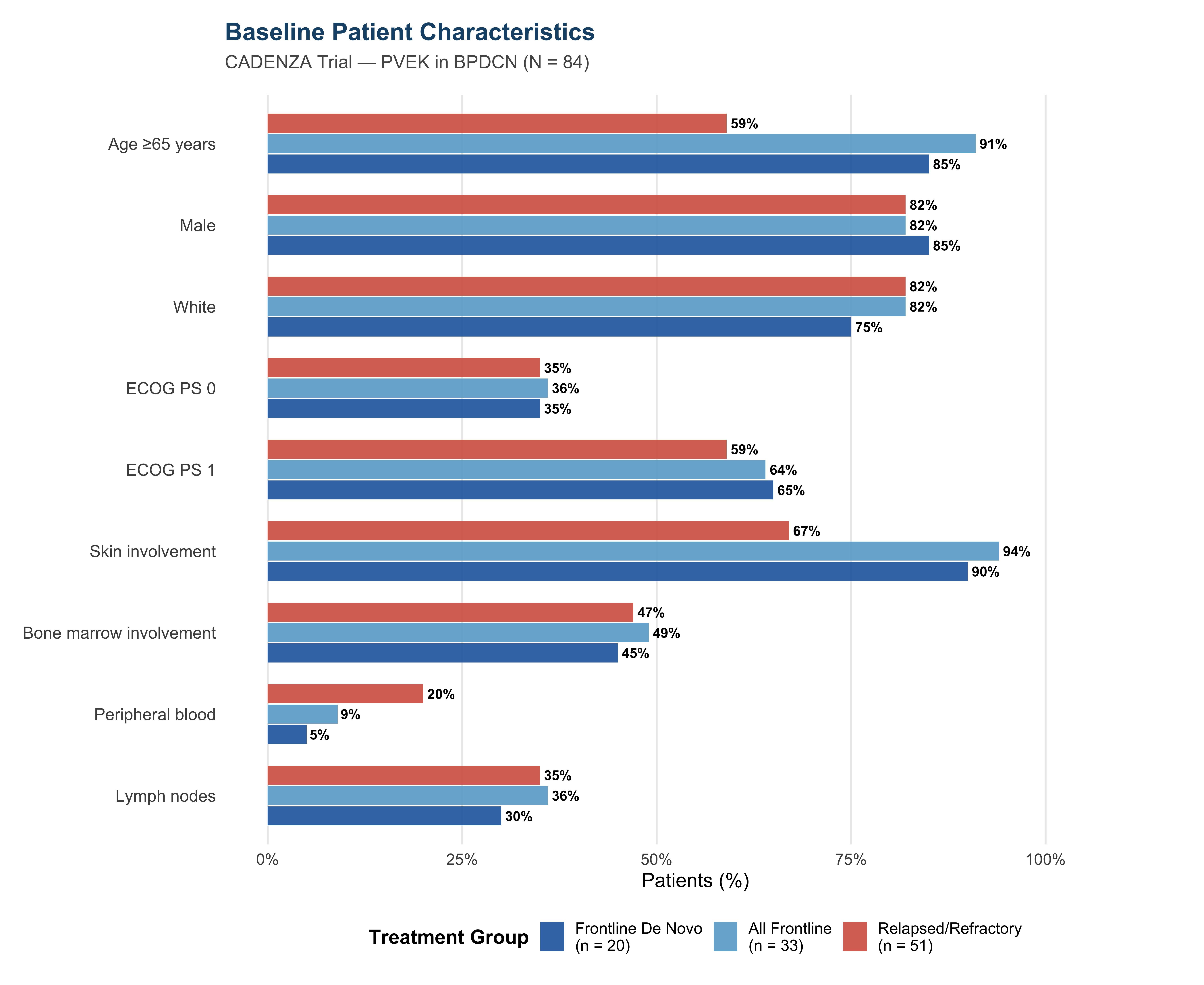
#| fig-cap: "Baseline demographic and clinical characteristics across treatment groups."
#| fig-height: 9
#| fig-width: 11
library(ggplot2)
library(dplyr)
library(tidyr)

# ── Demographics data from Table 1 ───────────────────────────────────
demo_data <- tibble(
  Characteristic = c(
    "Age ≥65 years", "Male", "White",
    "ECOG PS 0", "ECOG PS 1",
    "Skin involvement", "Bone marrow involvement",
    "Peripheral blood", "Lymph nodes"
  ),
  `Frontline De Novo\n(n = 20)` = c(85, 85, 75, 35, 65, 90, 45, 5, 30),
  `All Frontline\n(n = 33)`     = c(91, 82, 82, 36, 64, 94, 49, 9, 36),
  `Relapsed/Refractory\n(n = 51)` = c(59, 82, 82, 35, 59, 67, 47, 20, 35)
)

demo_long <- demo_data |>
  pivot_longer(-Characteristic, names_to = "Group", values_to = "Percentage") |>
  mutate(
    Characteristic = factor(Characteristic, levels = rev(demo_data$Characteristic)),
    Group = factor(Group, levels = c(
      "Frontline De Novo\n(n = 20)",
      "All Frontline\n(n = 33)",
      "Relapsed/Refractory\n(n = 51)"
    ))
  )

group_colors <- c(
  "Frontline De Novo\n(n = 20)" = "#2166ac",
  "All Frontline\n(n = 33)"     = "#67a9cf",
  "Relapsed/Refractory\n(n = 51)" = "#d6604d"
)

ggplot(demo_long, aes(x = Percentage, y = Characteristic, fill = Group)) +
  geom_col(position = position_dodge(width = 0.75), width = 0.7, alpha = 0.9) +
  geom_text(
    aes(label = paste0(Percentage, "%")),
    position = position_dodge(width = 0.75),
    hjust = -0.15, size = 3.2, fontface = "bold"
  ) +
  scale_fill_manual(values = group_colors) +
  scale_x_continuous(
    limits = c(0, 110),
    breaks = seq(0, 100, 25),
    labels = function(x) paste0(x, "%")
  ) +
  labs(
    title = "Baseline Patient Characteristics",
    subtitle = "CADENZA Trial — PVEK in BPDCN (N = 84)",
    x = "Patients (%)",
    y = NULL,
    fill = "Treatment Group"
  ) +
  theme_minimal(base_size = 13) +
  theme(
    plot.title = element_text(face = "bold", size = 16, color = "#1a5276"),
    plot.subtitle = element_text(size = 12, color = "#555555", margin = margin(b = 15)),
    legend.position = "bottom",
    legend.title = element_text(face = "bold"),
    panel.grid.major.y = element_blank(),
    panel.grid.minor = element_blank(),
    axis.text.y = element_text(size = 11),
    plot.margin = margin(15, 25, 15, 15)
  )
```
## Prior Therapies in Relapsed/Refractory Patients
```{python}
#| label: fig-prior-therapy
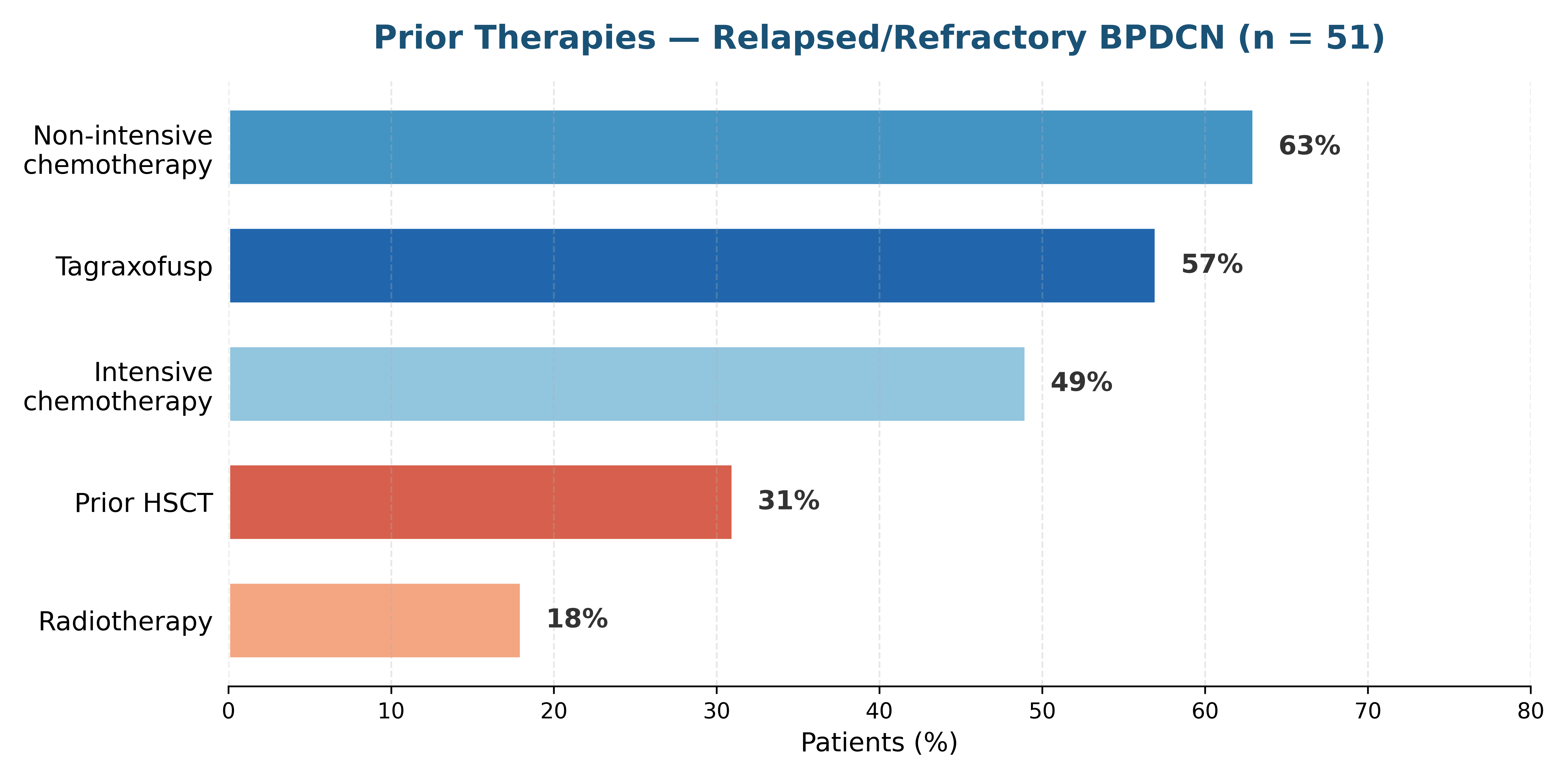
#| fig-cap: "Prior therapies received by patients with relapsed/refractory BPDCN (n = 51)."
#| fig-height: 5
import matplotlib.pyplot as plt
import matplotlib
matplotlib.rcParams['font.family'] = 'sans-serif'
import numpy as np

therapies = [
    'Non-intensive\nchemotherapy',
    'Tagraxofusp',
    'Intensive\nchemotherapy',
    'Prior HSCT',
    'Radiotherapy'
]
percentages = [63, 57, 49, 31, 18]

fig, ax = plt.subplots(figsize=(10, 5))

colors = ['#4393c3', '#2166ac', '#92c5de', '#d6604d', '#f4a582']

bars = ax.barh(
    range(len(therapies)), percentages,
    color=colors, edgecolor='white', linewidth=1.5, height=0.65
)

for bar, pct in zip(bars, percentages):
    ax.text(
        bar.get_width() + 1.5, bar.get_y() + bar.get_height()/2,
        f'{pct}%', va='center', ha='left', fontsize=12, fontweight='bold',
        color='#333333'
    )

ax.set_yticks(range(len(therapies)))
ax.set_yticklabels(therapies, fontsize=12)
ax.set_xlim(0, 80)
ax.set_xlabel('Patients (%)', fontsize=12)
ax.set_title(
    'Prior Therapies — Relapsed/Refractory BPDCN (n = 51)',
    fontsize=15, fontweight='bold', color='#1a5276', pad=15
)
ax.invert_yaxis()
ax.spines['top'].set_visible(False)
ax.spines['right'].set_visible(False)
ax.spines['left'].set_visible(False)
ax.tick_params(left=False)
ax.grid(axis='x', alpha=0.3, linestyle='--')

plt.tight_layout()
plt.show()
```
# Efficacy Results {#sec-efficacy}
## Response Rates
```{r}
#| label: fig-response
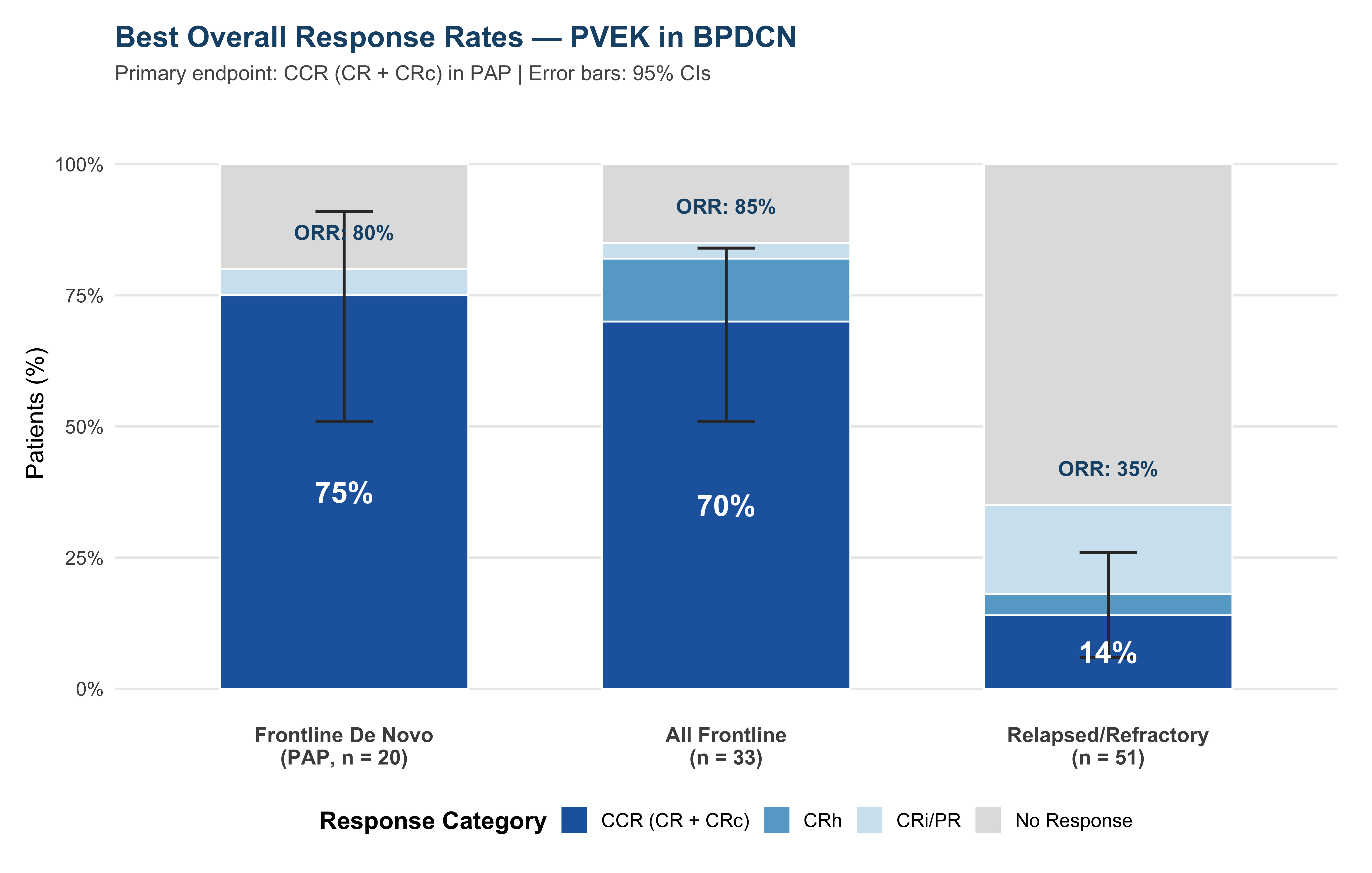
#| fig-cap: "Best overall response rates across patient populations. Error bars represent 95% Clopper–Pearson CIs for CCR."
#| fig-height: 7
#| fig-width: 11
library(ggplot2)
library(dplyr)
library(tidyr)

# ── Response data from Table 2 ───────────────────────────────────────
response_df <- tibble(
  Group = factor(c(
    "Frontline De Novo\n(PAP, n = 20)",
    "All Frontline\n(n = 33)",
    "Relapsed/Refractory\n(n = 51)"
  ), levels = c(
    "Frontline De Novo\n(PAP, n = 20)",
    "All Frontline\n(n = 33)",
    "Relapsed/Refractory\n(n = 51)"
  )),
  CCR  = c(75, 70, 14),
  CRh  = c(0, 12, 4),
  CRi_PR = c(5, 3, 17),
  No_Response = c(20, 15, 65),
  CCR_lower = c(51, 51, 6),
  CCR_upper = c(91, 84, 26)
)

# Reshape for stacked bars
resp_long <- response_df |>
  select(Group, CCR, CRh, CRi_PR, No_Response) |>
  pivot_longer(-Group, names_to = "Response", values_to = "Percentage") |>
  mutate(Response = factor(Response,
    levels = c("No_Response", "CRi_PR", "CRh", "CCR"),
    labels = c("No Response", "CRi/PR", "CRh", "CCR (CR + CRc)")
  ))

resp_colors <- c(
  "CCR (CR + CRc)" = "#2166ac",
  "CRh"            = "#67a9cf",
  "CRi/PR"         = "#d1e5f0",
  "No Response"    = "#e0e0e0"
)

# ORR labels
orr_labels <- tibble(
  Group = response_df$Group,
  ORR = c(80, 85, 35),
  y_pos = c(82, 87, 37)
)

ggplot(resp_long, aes(x = Group, y = Percentage, fill = Response)) +
  geom_col(width = 0.65, color = "white", linewidth = 0.5) +
  # CI error bars for CCR
  geom_errorbar(
    data = response_df,
    aes(x = Group, ymin = CCR_lower, ymax = CCR_upper, y = NULL, fill = NULL),
    inherit.aes = FALSE,
    width = 0.15, linewidth = 0.8, color = "#333333"
  ) +
  # CCR percentage label
  geom_text(
    data = response_df,
    aes(x = Group, y = CCR / 2, label = paste0(CCR, "%"),
        fill = NULL),
    inherit.aes = FALSE,
    color = "white", fontface = "bold", size = 6
  ) +
  # ORR annotation
  geom_text(
    data = orr_labels,
    aes(x = Group, y = y_pos + 5, label = paste0("ORR: ", ORR, "%"),
        fill = NULL),
    inherit.aes = FALSE,
    color = "#1a5276", fontface = "bold", size = 4.2
  ) +
  scale_fill_manual(values = resp_colors, name = "Response Category") +
  scale_y_continuous(
    limits = c(0, 105),
    breaks = seq(0, 100, 25),
    labels = function(x) paste0(x, "%")
  ) +
  labs(
    title = "Best Overall Response Rates — PVEK in BPDCN",
    subtitle = "Primary endpoint: CCR (CR + CRc) in PAP | Error bars: 95% CIs",
    x = NULL,
    y = "Patients (%)"
  ) +
  theme_minimal(base_size = 14) +
  theme(
    plot.title = element_text(face = "bold", size = 17, color = "#1a5276"),
    plot.subtitle = element_text(size = 12, color = "#555555", margin = margin(b = 15)),
    legend.position = "bottom",
    legend.title = element_text(face = "bold"),
    panel.grid.major.x = element_blank(),
    panel.grid.minor = element_blank(),
    axis.text.x = element_text(size = 12, face = "bold"),
    plot.margin = margin(15, 20, 15, 15)
  ) +
  guides(fill = guide_legend(reverse = TRUE))
```
::: {.callout-important}
## Primary Endpoint Met
The CCR rate in the PAP (75%; 95% CI, 51–91%) successfully rejected the null hypothesis of 10%, meeting the primary objective. The relapsed/refractory cohort (14%; 95% CI, 6–26%) also rejected its null hypothesis of 5%.
:::
## Overall Survival — Kaplan-Meier Analysis
```{r}
#| label: fig-km-survival
#| fig-cap: "Kaplan-Meier estimates of overall survival by treatment population. Shaded regions represent 95% confidence bands."
#| fig-height: 8
#| fig-width: 11
library(ggplot2)
library(dplyr)

# ── Reconstruct approximate KM curves from published at-risk tables ──
# PAP (n = 20): At-risk: 20, 20, 16, 14, 12, 11, 9, 5, 2, 0
# Events:         0,  0,  4,  6,  8,  8, 10,10,10,10
# Frontline (n=33): At-risk: 33,33,27,24,21,18,13,8,5,1
# R/R (n=51): At-risk: 51,40,22,15,12,10,6,5,5,2

# Approximate survival probabilities from the KM curves in Figure 2
km_data <- bind_rows(
  tibble(
    Time = c(0, 3, 6, 9, 12, 15, 18, 21, 24, 27),
    Survival = c(1.00, 1.00, 0.80, 0.70, 0.60, 0.55, 0.49, 0.49, 0.49, 0.49),
    Lower = c(1.00, 1.00, 0.58, 0.47, 0.36, 0.30, 0.26, 0.26, 0.26, 0.26),
    Upper = c(1.00, 1.00, 0.92, 0.85, 0.78, 0.74, 0.69, 0.69, 0.69, 0.69),
    Group = "Frontline De Novo (PAP)\nn = 20 | Median OS: 16.6 mo",
    n_risk = c(20, 20, 16, 14, 12, 11, 9, 5, 2, 0)
  ),
  tibble(
    Time = c(0, 3, 6, 9, 12, 15, 18, 21, 24, 27),
    Survival = c(1.00, 1.00, 0.82, 0.73, 0.64, 0.55, 0.44, 0.44, 0.44, 0.44),
    Lower = c(1.00, 1.00, 0.64, 0.55, 0.45, 0.36, 0.27, 0.27, 0.27, 0.27),
    Upper = c(1.00, 1.00, 0.92, 0.85, 0.78, 0.70, 0.60, 0.60, 0.60, 0.60),
    Group = "All Frontline\nn = 33 | Median OS: 16.6 mo",
    n_risk = c(33, 33, 27, 24, 21, 18, 13, 8, 5, 1)
  ),
  tibble(
    Time = c(0, 3, 6, 9, 12, 15, 18, 21, 24, 27),
    Survival = c(1.00, 0.78, 0.43, 0.29, 0.31, 0.24, 0.19, 0.19, 0.19, 0.19),
    Lower = c(1.00, 0.65, 0.30, 0.18, 0.18, 0.13, 0.09, 0.09, 0.09, 0.09),
    Upper = c(1.00, 0.88, 0.57, 0.43, 0.44, 0.37, 0.33, 0.33, 0.33, 0.33),
    Group = "Relapsed/Refractory\nn = 51 | Median OS: 5.8 mo",
    n_risk = c(51, 40, 22, 15, 12, 10, 6, 5, 5, 2)
  )
)

group_colors_km <- c(
  "Frontline De Novo (PAP)\nn = 20 | Median OS: 16.6 mo" = "#2166ac",
  "All Frontline\nn = 33 | Median OS: 16.6 mo" = "#4393c3",
  "Relapsed/Refractory\nn = 51 | Median OS: 5.8 mo" = "#d6604d"
)

ggplot(km_data, aes(x = Time, y = Survival, color = Group, fill = Group)) +
  # Confidence bands
  geom_ribbon(aes(ymin = Lower, ymax = Upper), alpha = 0.15, color = NA) +
  # KM step lines
  geom_step(linewidth = 1.3) +
  # Median OS reference lines
  geom_hline(yintercept = 0.5, linetype = "dashed", color = "grey50", linewidth = 0.5) +
  annotate("text", x = 0.5, y = 0.52, label = "50% survival",
           hjust = 0, size = 3.2, color = "grey40") +
  # Median OS markers
  geom_segment(aes(x = 16.6, xend = 16.6, y = 0, yend = 0.5),
               color = "#2166ac", linetype = "dotted", linewidth = 0.7,
               inherit.aes = FALSE) +
  geom_segment(aes(x = 5.8, xend = 5.8, y = 0, yend = 0.5),
               color = "#d6604d", linetype = "dotted", linewidth = 0.7,
               inherit.aes = FALSE) +
  annotate("text", x = 16.6, y = -0.04, label = "16.6", fontface = "bold",
           color = "#2166ac", size = 3.8) +
  annotate("text", x = 5.8, y = -0.04, label = "5.8", fontface = "bold",
           color = "#d6604d", size = 3.8) +
  scale_color_manual(values = group_colors_km) +
  scale_fill_manual(values = group_colors_km) +
  scale_x_continuous(breaks = seq(0, 27, 3), limits = c(0, 28)) +
  scale_y_continuous(
    breaks = seq(0, 1, 0.2),
    labels = scales::percent_format(),
    limits = c(-0.08, 1.05)
  ) +
  labs(
    title = "Overall Survival — Kaplan-Meier Estimates",
    subtitle = "PVEK 0.045 mg/kg Q3W in BPDCN | Data cutoff: October 2, 2024",
    x = "Time (months)",
    y = "Overall Survival Probability",
    color = "Population",
    fill = "Population"
  ) +
  theme_minimal(base_size = 14) +
  theme(
    plot.title = element_text(face = "bold", size = 17, color = "#1a5276"),
    plot.subtitle = element_text(size = 12, color = "#555555", margin = margin(b = 15)),
    legend.position = "bottom",
    legend.title = element_text(face = "bold"),
    legend.text = element_text(size = 10),
    panel.grid.minor = element_blank(),
    plot.margin = margin(15, 20, 15, 15)
  )
```
## Duration of Response and Bridge to SCT
```{r}
#| label: fig-dor-sct
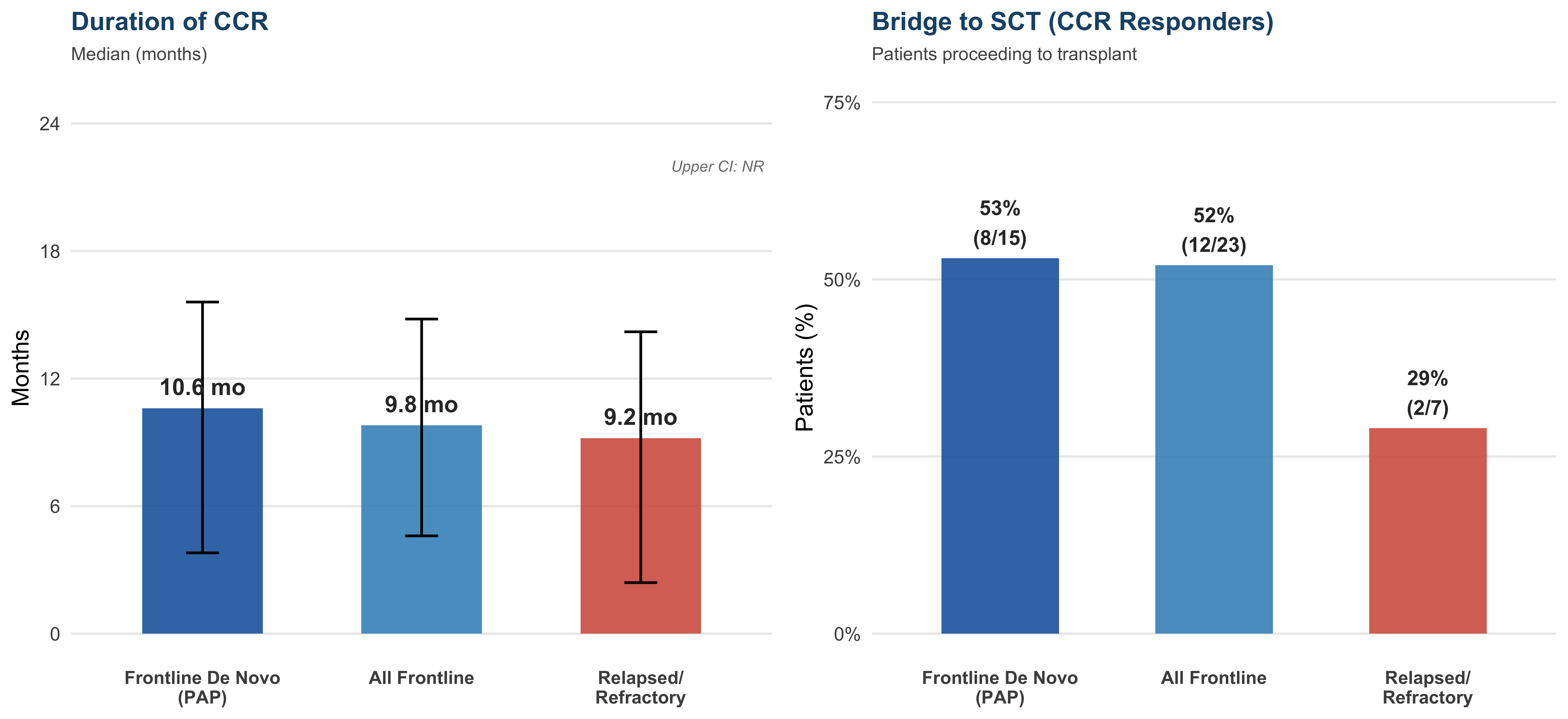
#| fig-cap: "Left: Duration of CCR across populations. Right: Rates of bridge to stem-cell transplant among CCR responders."
#| fig-height: 5.5
#| fig-width: 12
library(ggplot2)
library(dplyr)
library(tidyr)

# Panel A: Duration of Response
dor_data <- tibble(
  Group = factor(c(
    "Frontline De Novo\n(PAP)",
    "All Frontline",
    "Relapsed/\nRefractory"
  ), levels = c(
    "Frontline De Novo\n(PAP)",
    "All Frontline",
    "Relapsed/\nRefractory"
  )),
  Median_DoR = c(10.6, 9.8, 9.2),
  Lower = c(3.8, 4.6, 2.4),
  Upper = c(24, 24, 24),
  NR = c(TRUE, TRUE, TRUE)
)

p_dor <- ggplot(dor_data, aes(x = Group, y = Median_DoR, fill = Group)) +
  geom_col(width = 0.55, alpha = 0.9, show.legend = FALSE) +
  geom_errorbar(aes(ymin = Lower, ymax = ifelse(NR, Median_DoR + 5, Upper)),
                width = 0.15, linewidth = 0.7) +
  geom_text(aes(label = paste0(Median_DoR, " mo")),
            vjust = -0.8, fontface = "bold", size = 4.5, color = "#333333") +
  annotate("text", x = 3.35, y = 22, label = "Upper CI: NR",
           fontface = "italic", size = 3, color = "grey50") +
  scale_fill_manual(values = c("#2166ac", "#4393c3", "#d6604d")) +
  scale_y_continuous(limits = c(0, 25), breaks = seq(0, 24, 6)) +
  labs(
    title = "Duration of CCR",
    subtitle = "Median (months)",
    x = NULL, y = "Months"
  ) +
  theme_minimal(base_size = 13) +
  theme(
    plot.title = element_text(face = "bold", size = 14, color = "#1a5276"),
    plot.subtitle = element_text(size = 10, color = "#555555"),
    panel.grid.major.x = element_blank(),
    panel.grid.minor = element_blank(),
    axis.text.x = element_text(size = 10, face = "bold")
  )

# Panel B: Bridge to SCT among CCR responders
sct_data <- tibble(
  Group = factor(c(
    "Frontline De Novo\n(PAP)",
    "All Frontline",
    "Relapsed/\nRefractory"
  ), levels = c(
    "Frontline De Novo\n(PAP)",
    "All Frontline",
    "Relapsed/\nRefractory"
  )),
  SCT_pct = c(53, 52, 29),
  n = c(8, 12, 2),
  N = c(15, 23, 7)
)

p_sct <- ggplot(sct_data, aes(x = Group, y = SCT_pct, fill = Group)) +
  geom_col(width = 0.55, alpha = 0.9, show.legend = FALSE) +
  geom_text(aes(label = paste0(SCT_pct, "%\n(", n, "/", N, ")")),
            vjust = -0.3, fontface = "bold", size = 4, color = "#333333") +
  scale_fill_manual(values = c("#2166ac", "#4393c3", "#d6604d")) +
  scale_y_continuous(limits = c(0, 75), breaks = seq(0, 75, 25),
                     labels = function(x) paste0(x, "%")) +
  labs(
    title = "Bridge to SCT (CCR Responders)",
    subtitle = "Patients proceeding to transplant",
    x = NULL, y = "Patients (%)"
  ) +
  theme_minimal(base_size = 13) +
  theme(
    plot.title = element_text(face = "bold", size = 14, color = "#1a5276"),
    plot.subtitle = element_text(size = 10, color = "#555555"),
    panel.grid.major.x = element_blank(),
    panel.grid.minor = element_blank(),
    axis.text.x = element_text(size = 10, face = "bold")
  )

# Combine panels
library(gridExtra)
grid.arrange(p_dor, p_sct, ncol = 2)
```
## Landmark Survival Rates
```{python}
#| label: fig-landmark
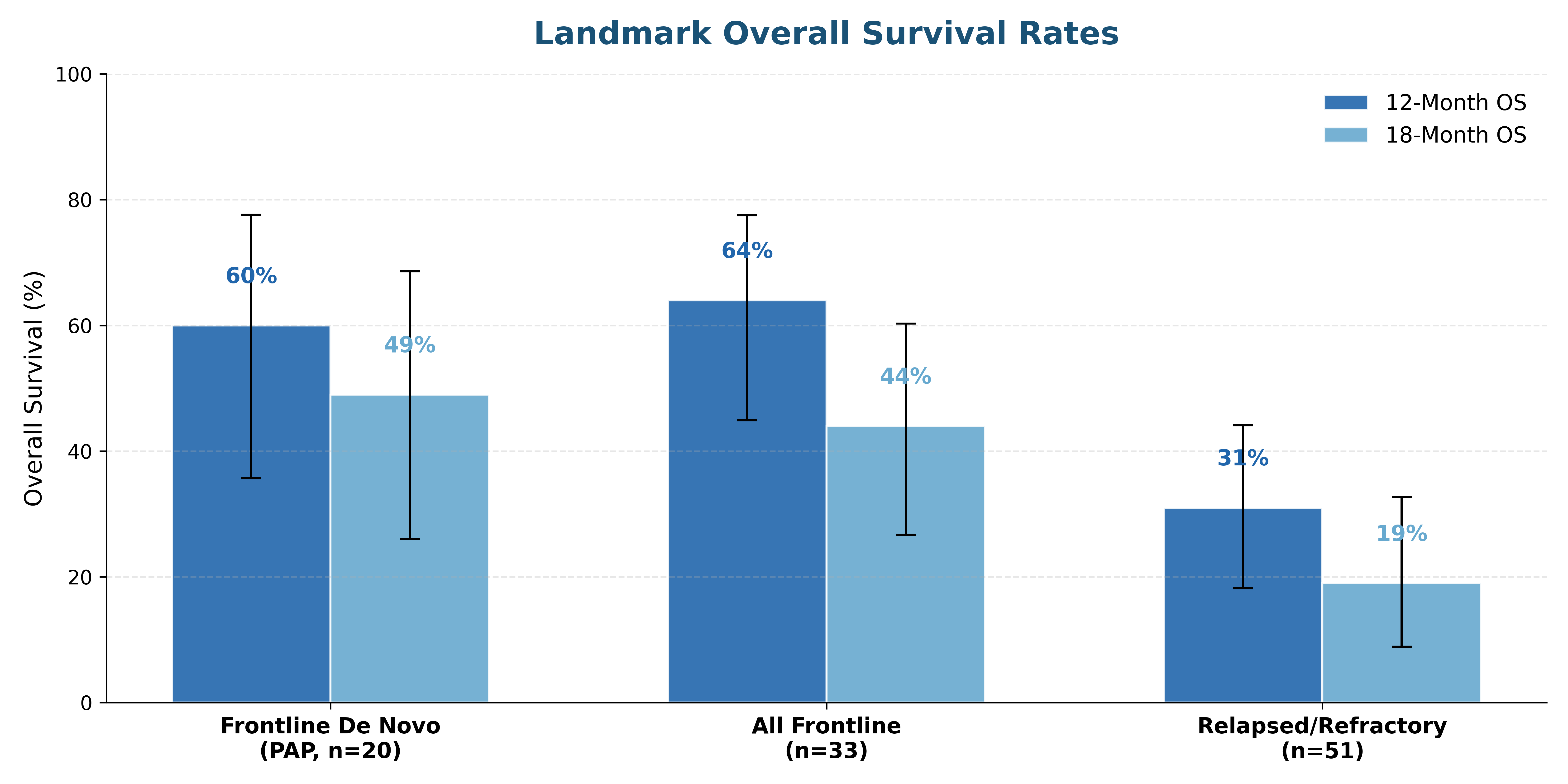
#| fig-cap: "Landmark overall survival rates at 12 and 18 months across treatment populations."
#| fig-height: 5.5
import matplotlib.pyplot as plt
import numpy as np

groups = ['Frontline De Novo\n(PAP, n=20)', 'All Frontline\n(n=33)', 'Relapsed/Refractory\n(n=51)']
os_12mo = [60, 64, 31]
os_18mo = [49, 44, 19]
ci_12mo = [(35.7, 77.6), (44.9, 77.5), (18.2, 44.1)]
ci_18mo = [(26.0, 68.6), (26.7, 60.3), (8.9, 32.7)]

x = np.arange(len(groups))
width = 0.32

fig, ax = plt.subplots(figsize=(11, 5.5))

err12 = [[v - lo for v, (lo, hi) in zip(os_12mo, ci_12mo)],
         [hi - v for v, (lo, hi) in zip(os_12mo, ci_12mo)]]
err18 = [[v - lo for v, (lo, hi) in zip(os_18mo, ci_18mo)],
         [hi - v for v, (lo, hi) in zip(os_18mo, ci_18mo)]]

bars1 = ax.bar(x - width/2, os_12mo, width, label='12-Month OS',
               color='#2166ac', alpha=0.9, edgecolor='white', linewidth=1,
               yerr=err12, capsize=5, error_kw={'linewidth': 1.2, 'color': '#333'})
bars2 = ax.bar(x + width/2, os_18mo, width, label='18-Month OS',
               color='#67a9cf', alpha=0.9, edgecolor='white', linewidth=1,
               yerr=err18, capsize=5, error_kw={'linewidth': 1.2, 'color': '#333'})

for bar, val in zip(bars1, os_12mo):
    ax.text(bar.get_x() + bar.get_width()/2, bar.get_height() + 6,
            f'{val}%', ha='center', va='bottom', fontweight='bold', fontsize=11,
            color='#2166ac')

for bar, val in zip(bars2, os_18mo):
    ax.text(bar.get_x() + bar.get_width()/2, bar.get_height() + 6,
            f'{val}%', ha='center', va='bottom', fontweight='bold', fontsize=11,
            color='#67a9cf')

ax.set_xticks(x)
ax.set_xticklabels(groups, fontsize=11, fontweight='bold')
ax.set_ylabel('Overall Survival (%)', fontsize=12)
ax.set_ylim(0, 100)
ax.set_title('Landmark Overall Survival Rates',
             fontsize=16, fontweight='bold', color='#1a5276', pad=15)
ax.legend(fontsize=11, frameon=False, loc='upper right')
ax.spines['top'].set_visible(False)
ax.spines['right'].set_visible(False)
ax.grid(axis='y', alpha=0.3, linestyle='--')

plt.tight_layout()
plt.show()
```
# Safety Profile {#sec-safety}
## Adverse Events Overview
```{python}
#| label: fig-ae-heatmap
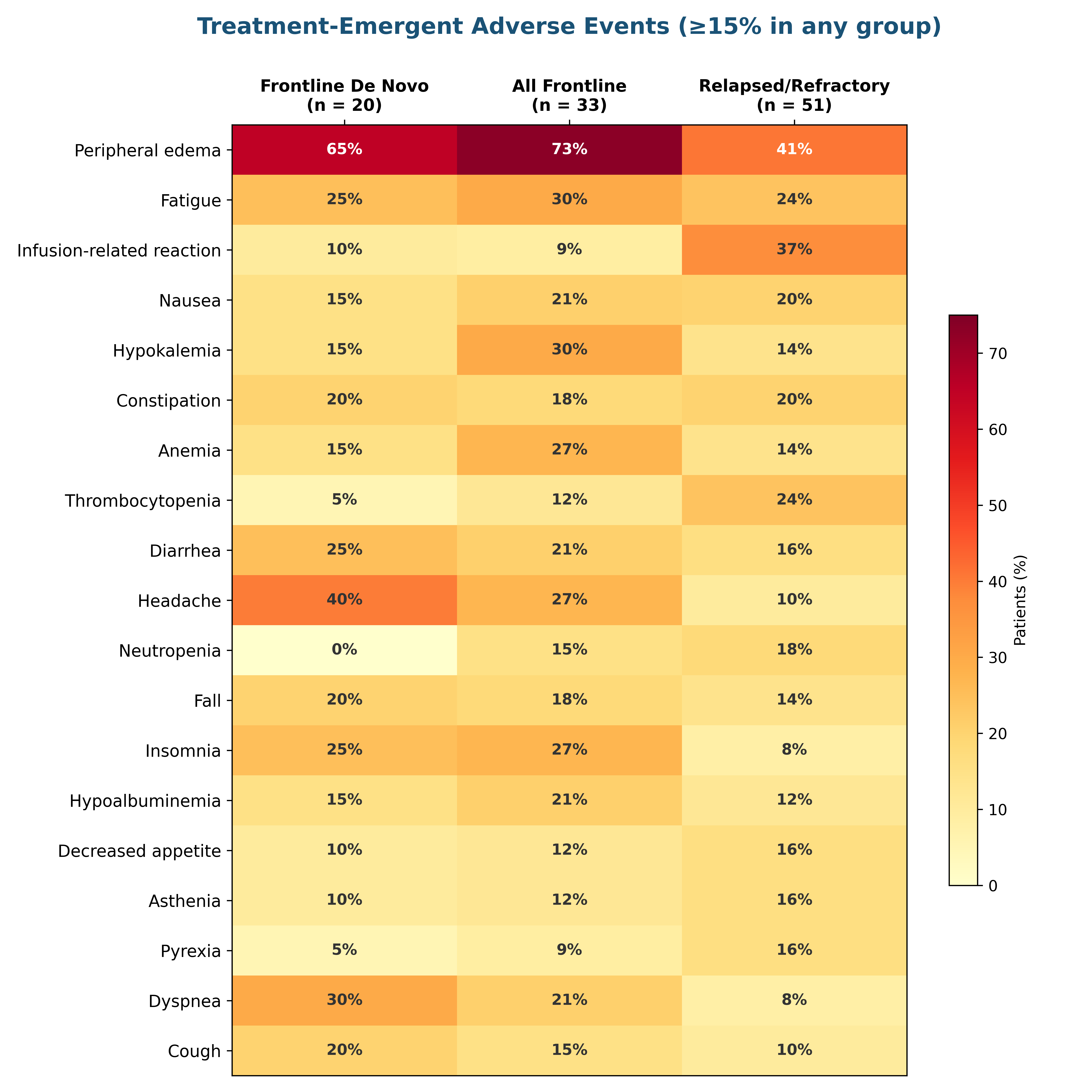
#| fig-cap: "Heatmap of treatment-emergent adverse events (≥15% in any group) by treatment population. Cell values represent the percentage of patients experiencing each event."
#| fig-height: 10
#| fig-width: 10
import matplotlib.pyplot as plt
import numpy as np
import seaborn as sns

aes = [
    'Peripheral edema', 'Fatigue', 'Infusion-related reaction',
    'Nausea', 'Hypokalemia', 'Constipation', 'Anemia',
    'Thrombocytopenia', 'Diarrhea', 'Headache', 'Neutropenia',
    'Fall', 'Insomnia', 'Hypoalbuminemia', 'Decreased appetite',
    'Asthenia', 'Pyrexia', 'Dyspnea', 'Cough'
]

frontline_denovo = [65, 25, 10, 15, 15, 20, 15, 5, 25, 40, 0, 20, 25, 15, 10, 10, 5, 30, 20]
all_frontline    = [73, 30, 9, 21, 30, 18, 27, 12, 21, 27, 15, 18, 27, 21, 12, 12, 9, 21, 15]
rr               = [41, 24, 37, 20, 14, 20, 14, 24, 16, 10, 18, 14, 8, 12, 16, 16, 16, 8, 10]

data = np.array([frontline_denovo, all_frontline, rr]).T

fig, ax = plt.subplots(figsize=(10, 10))

cmap = sns.color_palette("YlOrRd", as_cmap=True)

im = ax.imshow(data, cmap=cmap, aspect='auto', vmin=0, vmax=75)

for i in range(len(aes)):
    for j in range(3):
        val = data[i, j]
        color = 'white' if val > 40 else '#333333'
        ax.text(j, i, f'{val}%', ha='center', va='center',
                fontsize=10, fontweight='bold', color=color)

ax.set_xticks([0, 1, 2])
ax.set_xticklabels(
    ['Frontline De Novo\n(n = 20)', 'All Frontline\n(n = 33)',
     'Relapsed/Refractory\n(n = 51)'],
    fontsize=11, fontweight='bold'
)
ax.set_yticks(range(len(aes)))
ax.set_yticklabels(aes, fontsize=11)
ax.xaxis.set_ticks_position('top')
ax.xaxis.set_label_position('top')

cbar = plt.colorbar(im, ax=ax, shrink=0.6, label='Patients (%)')

ax.set_title('Treatment-Emergent Adverse Events (≥15% in any group)',
             fontsize=15, fontweight='bold', color='#1a5276', pad=60)

plt.tight_layout()
plt.show()
```
## Grade ≥3 Adverse Events
```{r}
#| label: fig-grade3-ae
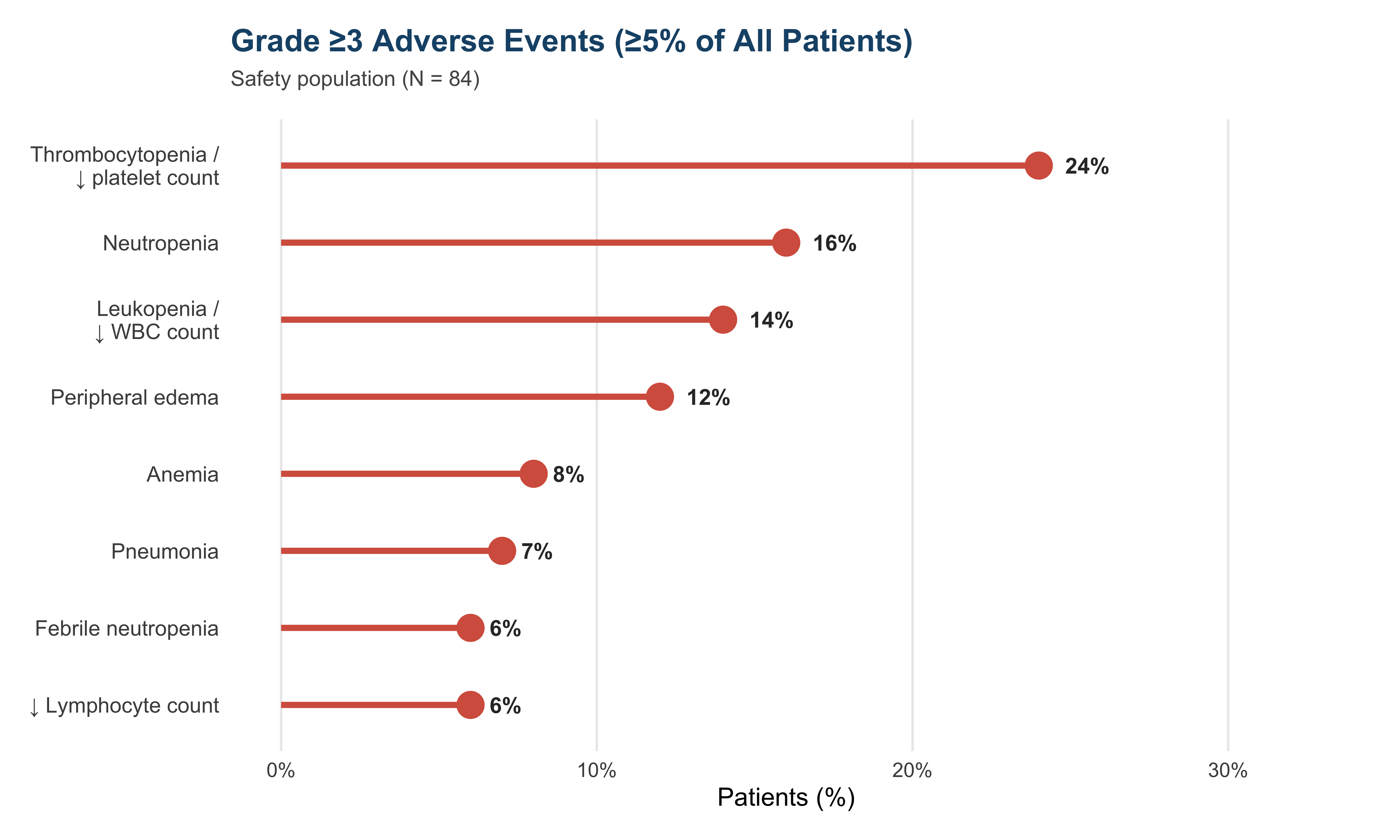
#| fig-cap: "Grade ≥3 adverse events reported in ≥5% of all patients (N = 84)."
#| fig-height: 6
#| fig-width: 10
library(ggplot2)
library(dplyr)

grade3_data <- tibble(
  AE = c(
    "Thrombocytopenia /\n↓ platelet count",
    "Neutropenia",
    "Leukopenia /\n↓ WBC count",
    "Peripheral edema",
    "Anemia",
    "Pneumonia",
    "Febrile neutropenia",
    "↓ Lymphocyte count"
  ),
  Percentage = c(24, 16, 14, 12, 8, 7, 6, 6)
) |>
  mutate(AE = factor(AE, levels = rev(AE)))

ggplot(grade3_data, aes(x = Percentage, y = AE)) +
  geom_segment(aes(x = 0, xend = Percentage, yend = AE),
               color = "#d6604d", linewidth = 1.5) +
  geom_point(size = 6, color = "#d6604d") +
  geom_text(aes(label = paste0(Percentage, "%")),
            hjust = -0.6, fontface = "bold", size = 4, color = "#333333") +
  scale_x_continuous(limits = c(0, 32), breaks = seq(0, 30, 10),
                     labels = function(x) paste0(x, "%")) +
  labs(
    title = "Grade ≥3 Adverse Events (≥5% of All Patients)",
    subtitle = "Safety population (N = 84)",
    x = "Patients (%)",
    y = NULL
  ) +
  theme_minimal(base_size = 13) +
  theme(
    plot.title = element_text(face = "bold", size = 16, color = "#1a5276"),
    plot.subtitle = element_text(size = 11, color = "#555555", margin = margin(b = 15)),
    panel.grid.major.y = element_blank(),
    panel.grid.minor = element_blank(),
    axis.text.y = element_text(size = 11),
    plot.margin = margin(15, 30, 15, 15)
  )
```
## Special Safety Topics
```{r}
#| label: tbl-safety-special
#| tbl-cap: "Summary of special safety events of interest."
library(knitr)

safety_special <- data.frame(
  Event = c(
    "Peripheral Edema",
    "Peripheral Edema",
    "Peripheral Edema",
    "Peripheral Edema",
    "Infusion-Related Reactions",
    "Infusion-Related Reactions",
    "Infusion-Related Reactions",
    "VOD (on-treatment)",
    "VOD (post-SCT)",
    "Capillary Leak Syndrome"
  ),
  Detail = c(
    "Median time to onset: 55 days (range 0–217)",
    "Most events (59%) first occurred in cycle 3",
    "70% received diuretic treatment; 56% resolved",
    "Only 1% led to treatment discontinuation",
    "Mostly mild-to-moderate (max grade 3: 4%)",
    "Median duration: 1 day (range 1–22)",
    "Preventable with prophylactic corticosteroids",
    "2 events (both resolved; led to discontinuation)",
    "5 of 19 post-SCT patients (4 with R/R BPDCN)",
    "No CLS events reported"
  )
)

kable(safety_special,
      col.names = c("Event", "Key Details"),
      align = c("l", "l"))
```
# Comparative Context {#sec-context}
```{python}
#| label: fig-comparison
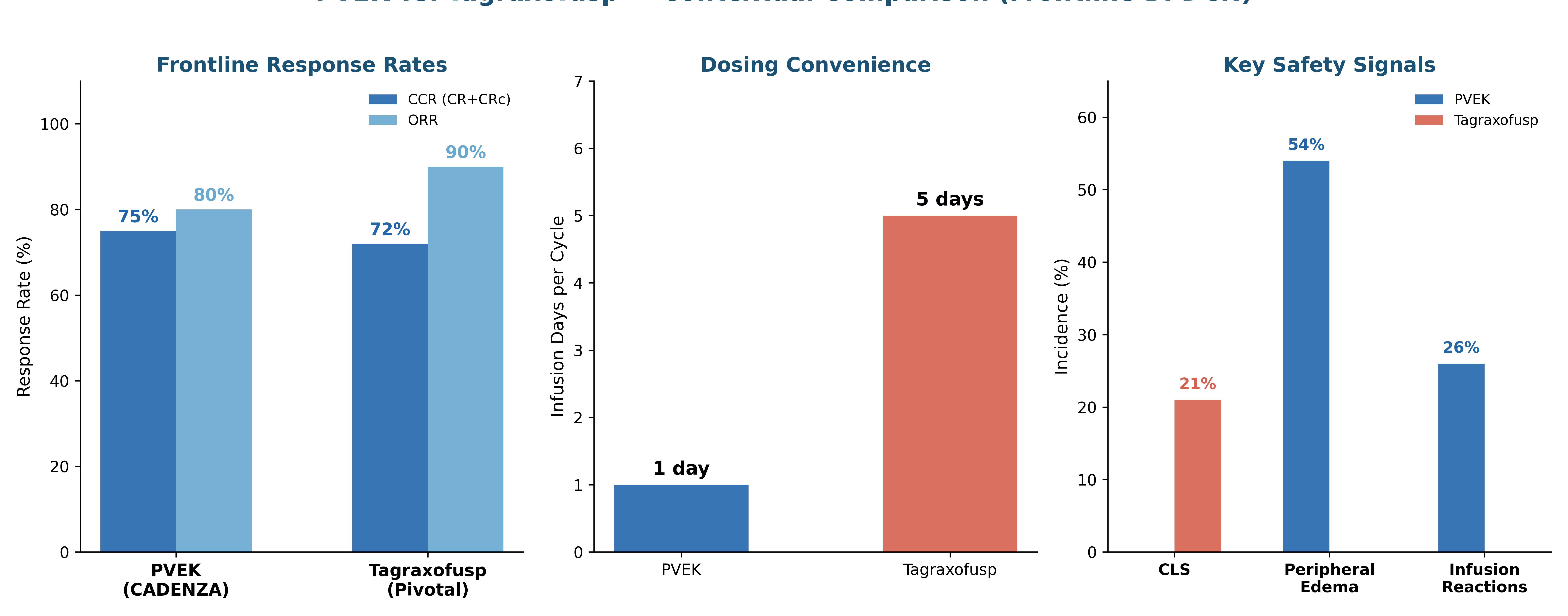
#| fig-cap: "Comparison of frontline response rates and key characteristics between PVEK (CADENZA) and tagraxofusp (pivotal study). Note: cross-trial comparisons should be interpreted with caution."
#| fig-height: 6
#| fig-width: 11
import matplotlib.pyplot as plt
import numpy as np

fig, axes = plt.subplots(1, 3, figsize=(14, 5.5))

# Panel A: CCR rates
drugs = ['PVEK\n(CADENZA)', 'Tagraxofusp\n(Pivotal)']
ccr = [75, 72]
orr = [80, 90]

x = np.arange(len(drugs))
w = 0.3
axes[0].bar(x - w/2, ccr, w, label='CCR (CR+CRc)', color='#2166ac', alpha=0.9)
axes[0].bar(x + w/2, orr, w, label='ORR', color='#67a9cf', alpha=0.9)

for i, (c, o) in enumerate(zip(ccr, orr)):
    axes[0].text(i - w/2, c + 2, f'{c}%', ha='center', fontweight='bold', fontsize=11, color='#2166ac')
    axes[0].text(i + w/2, o + 2, f'{o}%', ha='center', fontweight='bold', fontsize=11, color='#67a9cf')

axes[0].set_xticks(x)
axes[0].set_xticklabels(drugs, fontsize=11, fontweight='bold')
axes[0].set_ylabel('Response Rate (%)', fontsize=11)
axes[0].set_ylim(0, 110)
axes[0].set_title('Frontline Response Rates', fontsize=13, fontweight='bold', color='#1a5276')
axes[0].legend(fontsize=9, frameon=False)
axes[0].spines['top'].set_visible(False)
axes[0].spines['right'].set_visible(False)

# Panel B: Dosing comparison
labels = ['PVEK', 'Tagraxofusp']
infusion_days = [1, 5]
colors_dose = ['#2166ac', '#d6604d']
axes[1].bar(labels, infusion_days, color=colors_dose, width=0.5, alpha=0.9)
for i, v in enumerate(infusion_days):
    axes[1].text(i, v + 0.15, f'{v} day{"s" if v > 1 else ""}',
                ha='center', fontweight='bold', fontsize=12)
axes[1].set_ylabel('Infusion Days per Cycle', fontsize=11)
axes[1].set_ylim(0, 7)
axes[1].set_title('Dosing Convenience', fontsize=13, fontweight='bold', color='#1a5276')
axes[1].spines['top'].set_visible(False)
axes[1].spines['right'].set_visible(False)

# Panel C: Key AEs
ae_labels = ['CLS', 'Peripheral\nEdema', 'Infusion\nReactions']
pvek_ae = [0, 54, 26]
tagra_ae = [21, 0, 0]

x_ae = np.arange(len(ae_labels))
axes[2].bar(x_ae - w/2, pvek_ae, w, label='PVEK', color='#2166ac', alpha=0.9)
axes[2].bar(x_ae + w/2, tagra_ae, w, label='Tagraxofusp', color='#d6604d', alpha=0.9)
for i, (p, t) in enumerate(zip(pvek_ae, tagra_ae)):
    if p > 0:
        axes[2].text(i - w/2, p + 1.5, f'{p}%', ha='center', fontsize=10,
                    fontweight='bold', color='#2166ac')
    if t > 0:
        axes[2].text(i + w/2, t + 1.5, f'{t}%', ha='center', fontsize=10,
                    fontweight='bold', color='#d6604d')

axes[2].set_xticks(x_ae)
axes[2].set_xticklabels(ae_labels, fontsize=10, fontweight='bold')
axes[2].set_ylabel('Incidence (%)', fontsize=11)
axes[2].set_ylim(0, 65)
axes[2].set_title('Key Safety Signals', fontsize=13, fontweight='bold', color='#1a5276')
axes[2].legend(fontsize=9, frameon=False)
axes[2].spines['top'].set_visible(False)
axes[2].spines['right'].set_visible(False)

# Caveat
fig.text(0.5, -0.02,
         '⚠ Cross-trial comparisons should be interpreted with caution due to differences in study design and patient populations.',
         ha='center', fontsize=9, fontstyle='italic', color='#888888')

plt.suptitle('PVEK vs. Tagraxofusp — Contextual Comparison (Frontline BPDCN)',
             fontsize=16, fontweight='bold', color='#1a5276', y=1.03)
plt.tight_layout()
plt.show()
```
# Summary & Implications {#sec-summary}
```{r}
#| label: fig-summary
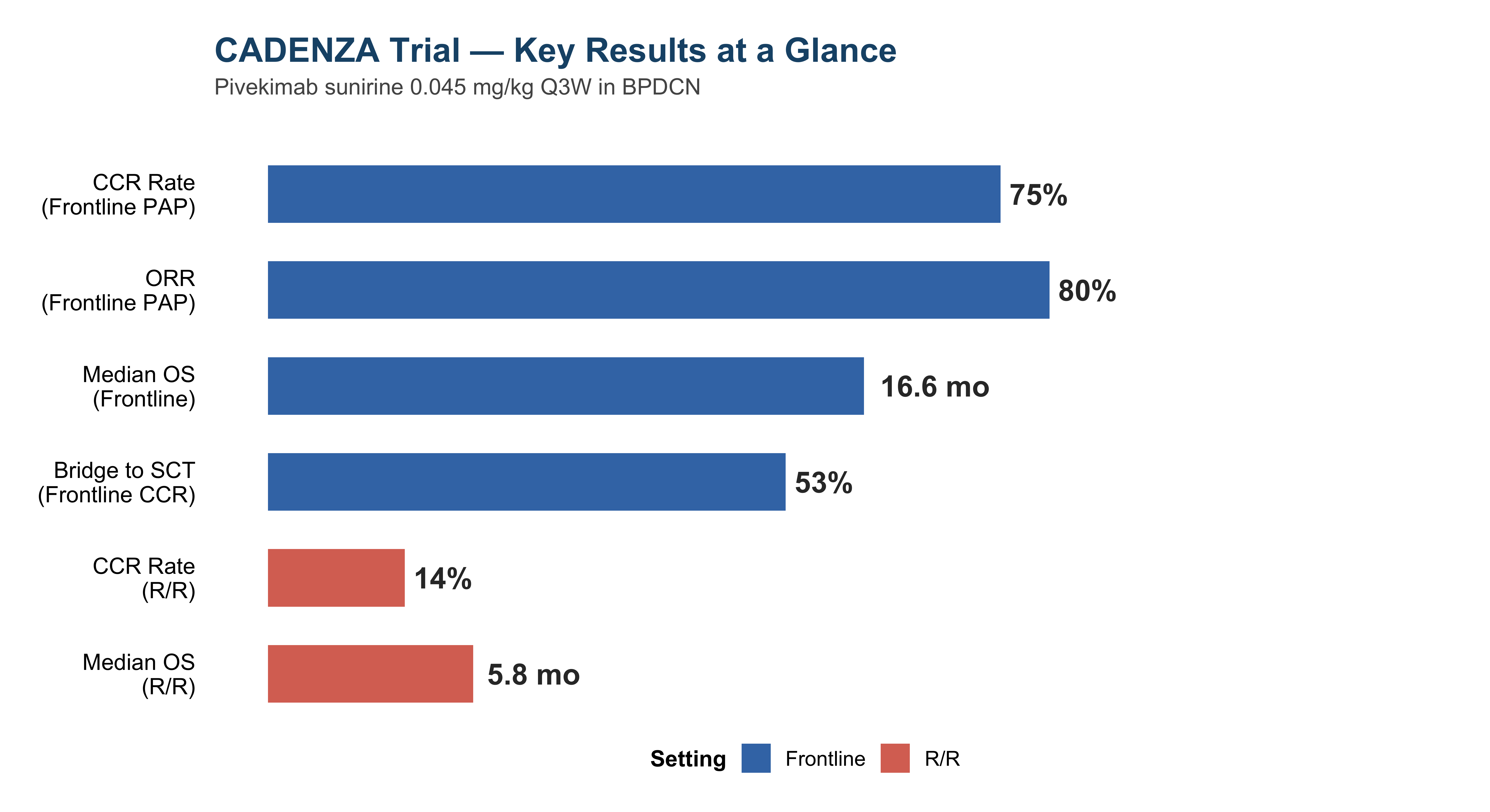
#| fig-cap: "Visual summary of key findings from the CADENZA trial of pivekimab sunirine in BPDCN."
#| fig-height: 6
#| fig-width: 11
library(ggplot2)

summary_data <- data.frame(
  Metric = factor(c(
    "CCR Rate\n(Frontline PAP)",
    "ORR\n(Frontline PAP)",
    "Median OS\n(Frontline)",
    "Bridge to SCT\n(Frontline CCR)",
    "CCR Rate\n(R/R)",
    "Median OS\n(R/R)"
  ), levels = rev(c(
    "CCR Rate\n(Frontline PAP)",
    "ORR\n(Frontline PAP)",
    "Median OS\n(Frontline)",
    "Bridge to SCT\n(Frontline CCR)",
    "CCR Rate\n(R/R)",
    "Median OS\n(R/R)"
  ))),
  Value = c(75, 80, 16.6, 53, 14, 5.8),
  Unit = c("%", "%", "months", "%", "%", "months"),
  Category = c("Frontline", "Frontline", "Frontline", "Frontline", "R/R", "R/R"),
  Display = c("75%", "80%", "16.6 mo", "53%", "14%", "5.8 mo"),
  bar_val = c(75, 80, 61, 53, 14, 21)  # Normalized for display
)

ggplot(summary_data, aes(x = bar_val, y = Metric, fill = Category)) +
  geom_col(width = 0.6, alpha = 0.9) +
  geom_text(aes(label = Display), hjust = -0.15,
            fontface = "bold", size = 5.5, color = "#333333") +
  scale_fill_manual(
    values = c("Frontline" = "#2166ac", "R/R" = "#d6604d"),
    name = "Setting"
  ) +
  scale_x_continuous(limits = c(0, 110)) +
  labs(
    title = "CADENZA Trial — Key Results at a Glance",
    subtitle = "Pivekimab sunirine 0.045 mg/kg Q3W in BPDCN",
    x = NULL, y = NULL
  ) +
  theme_void(base_size = 14) +
  theme(
    plot.title = element_text(face = "bold", size = 18, color = "#1a5276",
                              margin = margin(b = 5)),
    plot.subtitle = element_text(size = 12, color = "#555555",
                                 margin = margin(b = 20)),
    axis.text.y = element_text(size = 12, hjust = 1, margin = margin(r = 10)),
    legend.position = "bottom",
    legend.title = element_text(face = "bold", size = 12),
    legend.text = element_text(size = 11),
    plot.margin = margin(20, 50, 20, 20)
  )
```
::: {.callout-note appearance="minimal"}
## Clinical Implications
1. **High frontline efficacy**: 75% CCR in an older population (median age 74 years) with convenient Q3W outpatient dosing
2. **Effective bridge to transplant**: Over half of frontline responders proceeded to SCT
3. **No capillary leak syndrome**: A key differentiator from tagraxofusp
4. **Activity post-tagraxofusp**: Responses observed regardless of prior tagraxofusp exposure, potentially due to a different resistance mechanism
5. **Manageable safety**: Peripheral edema and infusion reactions were the most common AEs, predominantly low-grade and reversible
:::
---
::: {.callout-tip appearance="minimal"}
## Rendering This Document
To render this Quarto document, ensure the following are installed:
**R packages:**
```r
install.packages(c("ggplot2", "dplyr", "tidyr", "knitr", "gridExtra", "scales"))
```
**Python packages:**
```bash
pip install matplotlib numpy seaborn
```
**Render command:**
```bash
quarto render pvek_bpdcn_analysis.qmd
```
:::
*Source: Pemmaraju N, Marconi G, Montesinos P, et al. Pivekimab sunirine in blastic plasmacytoid dendritic cell neoplasm. J Clin Oncol. 2026. DOI: [10.1200/JCO-25-02083](https://doi.org/10.1200/JCO-25-02083). ClinicalTrials.gov: [NCT03386513](https://clinicaltrials.gov/ct2/show/NCT03386513).*